How SpaceX land first stage boosters
Animations and Mathematics
(Some of the technical details, as well as a neural network approach are detailed here.)I loosely followed a discussion on how SpaceX land their first stage rocket boosters, and thought I would try to understand how the boosters are controlled to land so accurately.
There are lots of different aspects to this question:
- How do they build something like this?
- How do they rotate the engines in flight?
- How do they work out exactly where the boosters are?
I'm just going to discuss how they work out what to wiggle and when, during flight, in order to get their rocket to land on its bottom.
I'm not affiliated with SpaceX, and my information is based on a handful of papers on the subject in the public domain. My aim is to explain the method in a way that does work, at least in my simulations, and is hopefully understandable.
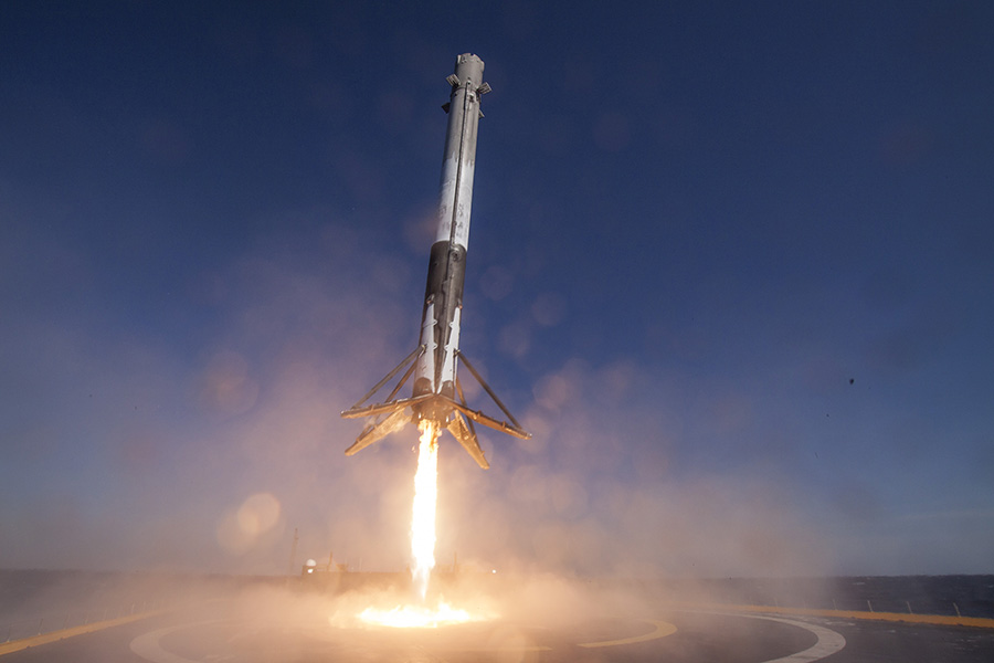
Image from SpaceX, with copyright waived. SpaceX make rockets that go to orbit. As far as we're concerned, these rockets have three bits:
- The main body that continues upwards into the sky.
- A booster (or two for the falcon heavy) that helps accelerate the main body, but only for the first two or three minutes.
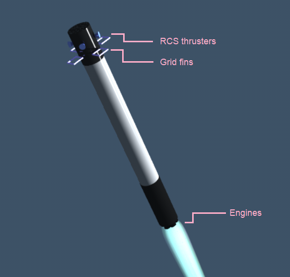
The booster
The booster is a 42m long cylinder with fuel inside, and nine engines on the bottom. It also has grid fins on the top and thrusters on the top. The booster is controlled in four ways:- The nine engines can have their thrust level adjusted.
- The nine engines are gimballed: their angle can be adjusted quickly in flight. If the engines are firing, then this produces a torque, rotating the vehicle.
- There are cold gas thrusters at the top of the vehicle. These are not very powerful, but are useful for rotating the vehicle in space.
- There are grid fins at the top of the vehicle. These can be rotated in flight to steer the vehicle.
The Task
The task here starts when the boosters detach from the main body of the rocket. They then become separate vehicles, which need to- turn around,
- accelerate in such a way that they end up on a trajectory ending at a suitable landing site,
- steer themselves through the atmosphere, so they stay on the right trajectory,
- decelerate at the end so that they are pretty much stopped when they hit the landing site,
- be more-or-less upright at the end of the flight so they don't fall over and explode.
How to solve it.
There are several ways to solve this, for instance:- Make a neural network and optimise it using a genetic algorithm: The neural networks that get closest to landing the thing replicate with mutation, whereas the neural networks that do worse get replaced.
- Neural networks with reinforcement learning, like this: landing_the_falcon_booster_with_reinforcement
-
Use Pontryagin's maximum principle. There is a differential equation that consists of the dynamics of the rocket and also some costate equations.
If you can find a solution to the differential equation, it tells you the optimal controls throughout the trajectory. I believe that this is, in theory, an elegant if somewhat complicated way to solve the problem, and involves simply
optimising or searching for the correct boundary conditions, which here may be a 5-Dimensional space.
This is a widely-known way to solve control problems, but I haven't personally used it. - Convex optimisation: You formulate the problem in such a way that it can be solved using a convex optimiser. This is apparently the in-favour approach and is discussed below. Compared to Pontragin's maximum principle, this is simple.
- Train a neural network to predict the convex optimisation's output. Like here.
Convex optimisers
An optimiser is a simple beast. It takes a list of statements about a problem, and spits out the solution to the problem. My aim here is to convince you that convex optimisers are not complicated to use or understand, and so this G-FOLD algorithm isn't actually all that difficult. For instance, you may tell it to find a series of 3 numbers, separated by 2 or less from the previous, with the first not more than 0, and and the last number as large as possible. It should then output 0,2,4 as the solution. All you have to do to use the optimiser is choose what to optimise, and write down two things: A scoring system, and a list of constraints. In this article, I'm going to set up the problem as follows:- The trajectory, in real life, is a continuous path. In this problem, I'm going to approximate it by positions, velocities, etc., at N equally spaced times. For instance, at t=0 seconds (now), at t=1 seconds, t=2, ...
- I'm going to choose that the thing I'm optimising is the velocities at each timepoint. This actually is equivalent to optimising the positions or the thrusts at each time, because given one of position, velocity, thrust, I can always work out the other two. It doesn't matter which I choose, but velocity, to me, seems simpler.
- I'm not going to model the rotation of the vehicle. It's assumed that it can jump from one angle to another instantly. This is a horrible approximation, but it seems to be what the other papers do too. This assumption is probably required for keeping the problem solvable by cone optimisers (which is what we're going to use).
| vx0 | The x-velocity at time 0 seconds |
| vy0 | The y-velocity at time 0 seconds |
| vz0 | The z-velocity at time 0 seconds |
| thrust0 | The absolute thrust at time 0 seconds |
| vx1 | The x-velocity at time 1 seconds |
| vy1 | The y-velocity at time 1 seconds |
| vz1 | The z-velocity at time 1 seconds |
| thrust1 | The absolute thrust at time 1 seconds |
| vx2 | The x-velocity at time 2 seconds |
| vy2 | The y-velocity at time 2 seconds |
| vz2 | The z-velocity at time 2 seconds |
| thrust2 | The absolute thrust at time 2 seconds |
| ... | ... |
| vxN-1 | The x-velocity at time N-1 seconds --- at the end of the flight |
| vyN-1 | The y-velocity at time N-1 seconds --- at the end of the flight |
| vzN-1 | The z-velocity at time N-1 seconds --- at the end of the flight |
| thrustN-1 | The absolute thrust at time N-1 seconds |
- Score = thrust0 + thrust1 + thrust2 + ... + thrustN-1
Rule 1: The initial velocity
Let's say we're on the booster, and we're moving downwards at 100 metres per second. The optimal useful trajectory has to have, at time t=0 (now), that vy = -100. Otherwise we can't use the trajectory: it's not our trajectory, it's just a trajectory.- vx0 = our actual x velocity.
- vy0 = our actual y velocity.
- vz0 = our actual z velocity.
Rule 2: The final velocity
We want to be stopped at the end of the trajectory.- vxN-1 = 0.
- vyN-1 = 0.
- vzN-1 = 0.
Rule 3: Position
During the first second, our average x velocity is (vx0 + vx1)*0.5 --- the average of the two velocities at either side of the second. We also know that the distance, in the x direction, that we'll move is going to be equal to this (because we have 1 second timesteps). We can add these 1-second steps up, and get the total distance we'll move over the trajectory:distance x = 0.5 vx0 + vx1 + vx2 + ... + vxN-2 + 0.5 vxN-1
Let us imagine now that we are at a known current height, and that the landing site is 100m in the x direction away, and level in the z direction. This gives us the following constraints:- distance x is between 95m and 105m.
- distance y is equal to our current height.
- distance z is between -5m and +5m.
Rule 4: Acceleration
At the moment, the optimiser could pick basically any trajectory it wanted: It could start here, move to the finish line, and stop there, and also declare that the total fuel is zero: We haven't told it anything about thrust or acceleration. We can tell the optimiser to be aware of how thrust works as follows. Let's pick the first timestep as an example:- sqrt((vx1 - vx0)2 + (vy1 - vy0 + g)2 + (vz1 - vz0)2) = thrust0
Rule 5: Max thrust
We have to limit the thrust to what the rocket can actually do.- thrusti <= MAX_THRUST
Let's see how this all works
Ok, so we have a way to calculate a trajectory. There are several things to look at: What is the trajectory, and more importantly, does a vehicle using this trajectory actually land? If we take an example test problem, and run it through the optimiser, we get one complete trajectory. This isn't the path that the rocket would take, it's just what the optimiser *thinks* will happen in its dreams: Just a plan. Next we need to see if it works in practice. Rather than build a 42m rocket, which planning laws prohibit, we can run a simulation. What we do is run a simulation with short timesteps (eg., 50 ms), and re-run the entire optimisation every second or so. The optimiser says something like "In the first second, accelerate along the (1.0,0.5,0.3) vector", and you can take that advice and use it for the first 20 or so timesteps. Note that the optimiser's useful output is just the thrust vector, it doesn't say how to fire the RCS thrusters to spin the vehicle. I've implemented a basic PD controller that won't allow the vehicle to tilt more than 45' that tries to orient the vehicle with future planned thrust directions. If we do that, we get the path the (simulated) rocket actually does take --- not just the optimisers plan: Note that the black line, in the video, is the plan that the rocket intends to take. Even the best-laid plans often go amiss, though, and these ones are no different: The optimiser isn't fed exactly the same physics as in real life: for instance, it doesn't know that the rocket tilt is unlikely to go outside 45', and it doesn't know that the thrust direction can't change instantly. As a result, the plan does change a fair bit during the flight. This is something that any real rocket will face in real life. Consequently, plans always do need to be re-optimised periodically. This does ok, but it's not upright when it hits its target, and when it hits the target, it doesn't really know it, so it keeps buzzing around re-planning how to get back to the target. We can improve this by adding a few more common-sense rules to the problem the optimiser solves each second.Other rules
You could add other rules, such as that the thrust has to be accelerating the vehicle roughly upwards: This prevents the rocket from wasting fuel by accelerating towards the target more than it should. This would happen if the number of timesteps is minimised. Another rule might be that the thrust direction shouldn't change too much from one second to the next (which I haven't implemented, but it wouldn't be difficult). Another quite extreme rule that I've added is that in the last second or two, the vehicle has to be travelling downwards (with almost no side-ways motion) at a certain speed.When you do these, and use that in the same old simulation as before, with the usual PD controller for the rocket RCS thrusters, you get this:
Comparison with SpaceX
The way I solved this differs from SpaceX in several ways. Firstly, I am trying to illustrate how convex optimisers are used to generate trajectory plans, and hopefully you can see how flexible the approach is. It is certain that the actual constraints used by spaceX are quite different to the ones I've chosen. For instance, some of the papers discuss constraining the trajectory to finish off inside a landing cone --- rather than a narrow landing cuboid that I have used --- which probably saves fuel. There are, however, a number of things that I've brushed over which will be quite a bit more complicated for SpaceX than for me:- Their engines can't be set to any level: They have to be either off, or going at a significant thrust, never just a tiny bit of thrust. This makes the problem more complicated.
- Their vehicle gets lighter as it uses fuel, meaning that the vehicle is more responsive at the end of the flight.
- The grid fins SpaceX use are probably harder to use than my RCS thrusters, and their RCS thrusters are less powerful than mine. This will make it harder to track the optimal trajectory.
- Their physics has uncertainty in it.
- They have to do the calculation in real time.
Literature review
Here's a quick literature review in an order that perhaps makes sense to the reader. No guarantee that this is in any way complete. These all seem to be free to the public. Lossless Convexification of Nonconvex Control Bound and Pointing Constraints of the Soft Landing Optimal Control Problem (Behçet Açıkme¸se, John M. Carson III, and Lars Blackmore) and Lossless convexification (Lars Blackmore)These two sites discuss, in particular, the way of overcoming what seems like an inconvexity in the problem due to various thrust limits that were ignored in my article. These two sites are of particular interest because they are by Lars Blackmore who was involved in the original development of the algorithm, and its use in actual landers. He works at SpaceX. G-FOLD: A Real-Time Implementable Fuel Optimal Large Divert Guidance Algorithm for Planetary Pinpoint Landing (by a team from the JPL)
This paper talks about the algorithm, called G-FOLD, in terms of what it can do for mars landers, pointing out how much better it is than the algorithms that were used half a century ago in the Apollo program. Fuel-Optimal Spacecraft Guidance for Landing in Planetary Pits (Neal S. Bhasin)
This gives a lot more mathematical detail about how convex optimisation can solve trajectories, and has some cool pictures, and is also focussed on landing on Mars and places like that. Landing Rockets Propulsively (Jonny Hyman)
This has a video of G-Fold being used in KSP. ECOS: An SOCP Solver for Embedded Systems (Alexander Domahidi, Eric Chu and Stephen Boyd)
This is the conical solver that I used in this article. Some of the technical details, as well as a neural network approach are detailed here.
Other Articles:
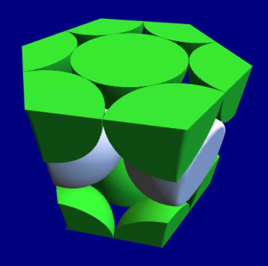
Three Crystal StructuresA ThreeJS model of three crystal structures |
|
|
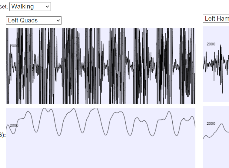
BodyWorks: EMG AnalysisA page with a javascript application where you can interact with EMG data using various filters. |
AtmosphereA simple demo of a simulation of an atmosphere. It looks quite cool, but there's not a lot you can do with it yet, and the physics isn't yet all that accurate. |
|