How to simulate fractal ice crystal growth in Python
Fourier transforms and density functions
September 2021

This is an article taken from the physics book I'm writing. I'm using the example of water molecules diffusing onto an ice crystal, in order to illustrate how Fourier transforms can be used to solve a diffusion equation. I chose python for this because it's probably simpler to use than Kotlin for this, and more people know it. I thought that this article may be a good standalone article for the website, so here it is.
Ice crystals might grow when water molecules, previously free in the air, land on an ice crystal and stick. If you imagine that the surface of the crystal has jagged peaks and deep valleys, a wandering water molecule is far more likely to hit a peak than a valley, and so the peaks grow faster.
This makes it unlikely that the crystal will grow as a perfect sphere, and indeed they end up with spines and spikes all around them.
Although this story is heavily simplified, simulating how this works does typically give fractals that resemble snowflake ice crystals.
We can simulate this qualitatively with a particle simulation as follows:
# Keep track of what is ice and what's not:
A : 2d Array from -alot to +alot
A[0,0] = 1

while True:
    place a particle at (x:Int,y:Int) somewhere random but far away.
    while True:
        move the particle a small distance randomly, updating x and y
        if A[x,y]:
            A[previous x, previous y] = 1
            break
This gives us a fractal shape like this:
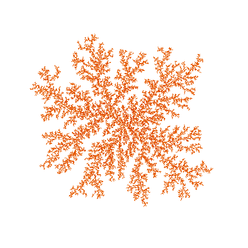
This has some of the branching that real ice crystals in snowflakes have, but it is far more random than real life. There are lots of reasons for this, but one part of it is that simulating individual particles is just too random. In real life, these crystals may have millions of trillions of water molecules in them, which is more than we could simulate individually.
So how do we tackle this? We can model the particle density as a 2- or 3-Dimensional array, and model diffusion on that array.
Diffusion can be modelled with a convolution between the particle density array and a Green's function - a gaussian kernel. Basically, if you know the particle density, ρ(x,y,t), at time t, then the particle density at time t + 𝛿t is given by the following:
ρ(x,y,t + 𝛿t) = ρ(x,y,t) ∗ G,
where G(x,y) = exp (-(x^2 + y^2) / s^2), and ∗ is the convolution operator.
To simulate the rest of the process, we also need to set the density to zero anywhere where there is an ice crystal --- to model the idea that any particles hitting the crystal will stick. We also need to allow the crystal to grow into adjacent cells according to adjacent particle density.
There is a fair bit more to explain here, but It's probably best for the interested reader to get a jupyter notebook up and running, and just copy the following code in and play around with it:
Note that the convolutions are done using Fourier transforms, which is efficient, and benefits from being able to take one of the Fourier transforms out of the inner loop.
import numpy as np
import math
from PIL import Image
from tqdm import tqdm


n = 800

# This
def getSmoother(n):
    smoother = np.zeros([n, n])
    smoother[0, 0] = 1
    smoother[0, 1] = 1
    smoother[1, 0] = 1
    smoother[-1, 0] = 1
    smoother[0, -1] = 1
    smoother[1, -1] = 1
    smoother[-1, 1] = 1
    return smoother


def getG(n):
    G = np.zeros([n, n])
    for i in range(n):
        for j in range(n):
            i2 = i
            j2 = j
            if i2 > n/2:
                i2 -= n
            if j2 > n/2:
                j2 -= n
            # we're on a hexagonal grid, so this
            # is the x displacement for two tiles
            dx = i2 + 0.5 * j2
            # and the y displacement
            dy = j2 * math.sqrt(3)/2
            r = math.sqrt(dx*dx+dy*dy)
            G[i, j] = math.exp(-r*r/8)
    G = G / np.sum(np.sum(G))
    return G


frame = 0
def save(A):
    global frame
    B = A * 0.2
    n = len(A)
    B[B < 0.01] = 0

    # This handles the hexagonal grid, somewhat approximately:
    B = np.array(
        [B[i, range((n // 2 - i // 2), (n - i // 2), 1)] for i in range(n // 4, (3 * n) // 4, 1) if (i % 5) != 0])

    def red(x):
        return np.uint(math.exp(-x * 4.0) * 255)

    def green(x):
        return np.uint(math.exp(-x) * 255)

    def blue(x):
        return np.uint(math.exp(-x / 4.0) * 255)

    col = [[[red(x), green(x), blue(x), 255] for x in y] for y in B]
    im = Image.fromarray(np.uint8(col))
    im.save(f"frames/im{10000 + frame}.png")
    frame += 1


def main():
    n = 1200
    A = np.zeros([n, n])
    A[n//2, n//2] = 1
    G = getG(n)
    smoother = getSmoother(n)
    rho = np.ones([n, n])

    sf = np.fft.fft2(smoother)
    gf = np.fft.fft2(G)
    for i in tqdm(range(5000)):
        B = A.copy()
        B[B < 1] = 0
        B[B > 1] = 1

        A2 = np.fft.ifft2(np.multiply(sf, np.fft.fft2(B))).real
        A2[A2 > 0.9] = 1
        A2[A2 < 0.9] = 0
        A += A2 * (rho * 0.5)
        A[A > 5] = 5

        rho[A > 0.5] = 0
        rho = np.fft.ifft2(np.multiply(gf, np.fft.fft2(rho))).real
        rho = rho / np.mean(np.mean(rho)) + np.random.randn(n, n) * 0.02
        if (i%5)==0:
            save(A)
    save(A)


if __name__ == '__main__':
    main()
Summary
If anyone wants a simple python code that demonstrates using Fourier transforms to grow an ice crystal, here it is.
Enjoy
Other Articles:
Mars Re-EntryA ThreeJS simulation of Mars re-entry in a spaceship. |
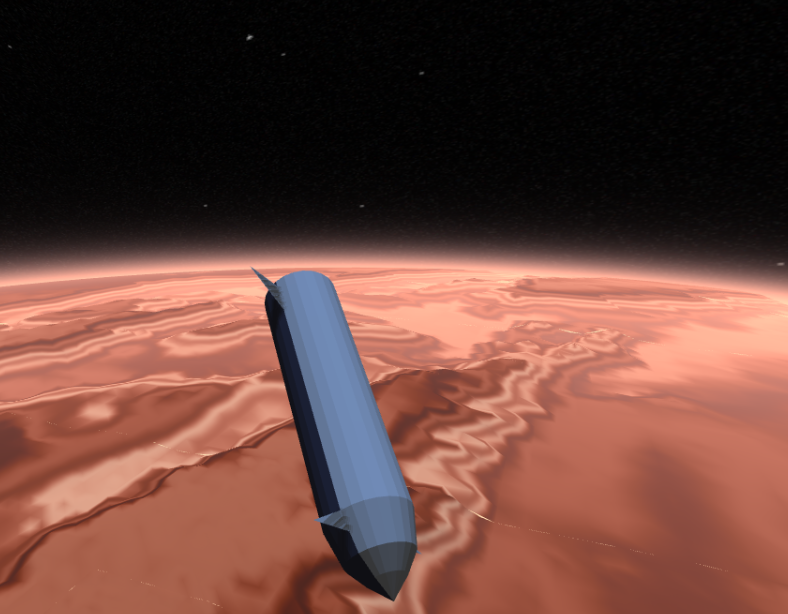
|
|
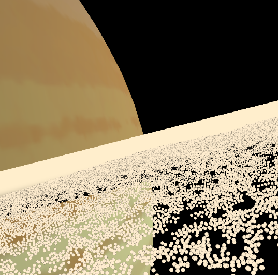
Saturn's ringsA simulation of Saturn's rings --- a few thousand particles are simulated, in a repeating tiled region. You use the mouse and keys to fly in it. |